 Русский
Introduction to pandas: data analytics in Python
pandas probably is the most popular library for data analysis in Python programming language. This library is a high-level abstraction over low-level NumPy which is written in pure C. I use pandas on a daily basis and really enjoy it because of its eloquent syntax and rich functionality. Hope this note will help you dive into data analysis realm with Python and pandas.
DataFrame and Series
In order to master pandas you have to start from scratch with two main data structures: DataFrame and Series. If you don't understand them well you won't understand pandas.
Series
Series is an object which is similar to Python built-in list data structure but differs from it because it has associated label with each element or so-called index. This distinctive feature makes it look like associated array or dictionary (hashmap representation).
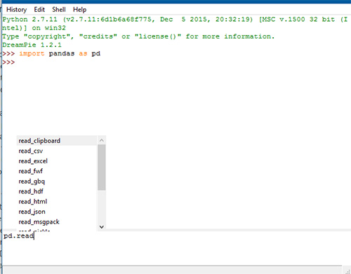
>>> import pandas as pd
>>> my_series = pd.Series([5, 6, 7, 8, 9, 10])
>>> my_series
0     5
1     6
2     7
3     8
4     9
5    10
dtype: int64
>>>
Take a look at the output above and you will see that index is leftward and values are to the right. If index is not provided explicitly, then pandas creates RangeIndex starting from 0 to N-1, where N is a total number of elements. Moreover, each Series object has data type (dtype), in our case data type is int64.
Series has attributes to extract its values and index:
>>> my_series.index
RangeIndex(start=0, stop=6, step=1)
>>> my_series.values
array([ 5,  6,  7,  8,  9, 10], dtype=int64)
You can retrieve elements by their index number:
>>> my_series[4]
9
You can provide index (labels) explicitly:
>>> my_series2 = pd.Series([5, 6, 7, 8, 9, 10], index=['a', 'b', 'c', 'd', 'e', 'f'])
>>> my_series2['f']
10
It is easy to retrieve several elements by their indexes or make group assignment:
>>> my_series2[['a', 'b', 'f']]
a     5
b     6
f    10
dtype: int64
>>> my_series2[['a', 'b', 'f']] = 0
>>> my_series2
a    0
b    0
c    7
d    8
e    9
f    0
dtype: int64
Filtering and math operations are easy as well:
>>> my_series2[my_series2 > 0]
c    7
d    8
e    9
dtype: int64
>>> my_series2[my_series2 > 0] * 2
c    14
d    16
e    18
dtype: int64
Because Series is very similar to dictionary, where key is an index and value is an element, we can do this:
>>> my_series3 = pd.Series({'a': 5, 'b': 6, 'c': 7, 'd': 8})
>>> my_series3
a    5
b    6
c    7
d    8
dtype: int64
>>> 'd' in my_series3
True
Also Series object and its index have name attributes, so you can label them:
>>> my_series3.name = 'numbers'
>>> my_series3.index.name = 'letters'
>>> my_series3
letters
a    5
b    6
c    7
d    8
Name: numbers, dtype: int64
Index can be changed "on fly" by assigning list to index attribute:
>>> my_series3.index = ['A', 'B', 'C', 'D']
>>> my_series3
A    5
B    6
C    7
D    8
Name: numbers, dtype: int64
But bear in mind that the length of the list should be equal to the number of elements inside Series and also labels have to be unique.
DataFrame
Simply said, DataFrame is a table. It has rows and columns. Each column in a DataFrame is a Series object, rows consist of elements inside Series.
DataFrame can be constructed using built-in Python dicts:
>>> df = pd.DataFrame({
...     'country': ['Kazakhstan', 'Russia', 'Belarus', 'Ukraine'],
...     'population': [17.04, 143.5, 9.5, 45.5],
...     'square': [2724902, 17125191, 207600, 603628]
... })
>;>> df
   country  population    square
0  Kazakhstan       17.04   2724902
1      Russia      143.50  17125191
2     Belarus        9.50    207600
3     Ukraine       45.50    603628
In order to make sure that each column is a Series object let's do this:
>>> df['country']
0    Kazakhstan
1        Russia
2       Belarus
3       Ukraine
Name: country, dtype: object
>>> type(df['country'])
<class 'pandas.core.series.Series'>
DataFrame object has 2 indexes: column index and row index. If you do not provide row index explicitly, pandas will create RangeIndex from 0 to N-1, where N is a number of rows inside DataFrame.
>>> df.columns
Index([u'country', u'population', u'square'], dtype='object')
>>> df.index
RangeIndex(start=0, stop=4, step=1)
Our table/DataFrame has 4 elements from 0 to 3.
Accessing elements by Index:
There are numerous ways to provide row index explicitly, for example you can provide index when creating a DataFrame or do it “on the fly” during runtime:
>>> df = pd.DataFrame({
...     'country': ['Kazakhstan', 'Russia', 'Belarus', 'Ukraine'],
...     'population': [17.04, 143.5, 9.5, 45.5],
...     'square': [2724902, 17125191, 207600, 603628]
... }, index=['KZ', 'RU', 'BY', 'UA'])
>>> df
       country  population    square
KZ  Kazakhstan       17.04   2724902
RU      Russia      143.50  17125191
BY     Belarus        9.50    207600
UA     Ukraine       45.50    603628
>>> df.index = ['KZ', 'RU', 'BY', 'UA']
>>> df.index.name = 'Country Code'
>>> df
                 country  population    square
Country Code
KZ            Kazakhstan       17.04   2724902
RU                Russia      143.50  17125191
BY               Belarus        9.50    207600
UA               Ukraine       45.50    603628
Besides creating an index I have also named it as Country Code. Series object will also have the same index as DataFrame has:
>>> df['country']
Country Code
KZ    Kazakhstan
RU        Russia
BY       Belarus
UA       Ukraine
Name: country, dtype: object
Row access using index can be performed in several ways:
- using .loc and providing index label
- using .iloc and providing index number
>>> df.loc['KZ']
country       Kazakhstan
population         17.04
square           2724902
Name: KZ, dtype: object
>>> df.iloc[0]
country       Kazakhstan
population         17.04
square           2724902
Name: KZ, dtype: object
Selection of particular rows and columns can be performed this way:
>>> df.loc[['KZ', 'RU'], 'population']
Country Code
KZ     17.04
RU    143.50
Name: population, dtype: float64
.loc takes 2 arguments: index list and column list, slicing operation is supported as well:
>>> df.loc['KZ':'BY', :]
                 country  population    square
Country Code
KZ            Kazakhstan       17.04   2724902
RU                Russia      143.50  17125191
BY               Belarus        9.50    207600
Filtering is performed using so-called Boolean arrays:
>>> df[df.population > 10][['country', 'square']]
                 country    square
Country Code
KZ            Kazakhstan   2724902
RU                Russia  17125191
UA               Ukraine    603628
By the way, columns can be accessed using attribute or Python dict notation, for example df.population and df[‘population’] are the same operations.
If you want to reset index, no problem:
>>> df.reset_index()
  Country Code     country  population    square
0           KZ  Kazakhstan       17.04   2724902
1           RU      Russia      143.50  17125191
2           BY     Belarus        9.50    207600
3           UA     Ukraine       45.50    603628
By default when you manipulate a DataFrame, pandas will return a new instance (the old one will not be affected).
Let’s add new column with population density:
>>> df['density'] = df['population'] / df['square'] * 1000000
>>> df
                 country  population    square    density
Country Code
KZ            Kazakhstan       17.04   2724902   6.253436
RU                Russia      143.50  17125191   8.379469
BY               Belarus        9.50    207600  45.761079
UA               Ukraine       45.50    603628  75.377550
Don’t like new column? OK, let’s delete it:
>>> df.drop(['density'], axis='columns')
                 country  population    square
Country Code
KZ            Kazakhstan       17.04   2724902
RU                Russia      143.50  17125191
BY               Belarus        9.50    207600
UA               Ukraine       45.50    603628
If you are too lazy to type drop... you can use del df[‘density’]
Rename it!
>>> df = df.rename(columns={'Country Code': 'country_code'})
>>> df
  country_code     country  population    square
0           KZ  Kazakhstan       17.04   2724902
1           RU      Russia      143.50  17125191
2           BY     Belarus        9.50    207600
3           UA     Ukraine       45.50    603628
In our renaming example make sure that you dropped the index otherwise invoking rename method will have no effect.
Reading and Writing
pandas supports many popular file formats including CSV, XML, HTML, Excel, SQL, JSON many more (check out official docs).
But usually (in my practice) I use CSV files. For example, if you want to save our previous DataFrame run this:
>>> df.to_csv('filename.csv')to_csvmethod takes many arguments (for example, separator character), if you want to know more make sure to check official documentation.
We have saved our DataFrame, but what about reading data? No problem:
>>> df = pd.read_csv('filename.csv', sep=',')Named argument sep points to a separator character in CSV file called filename.csv. There are many different ways to construct DataFrame from external sources, for example using read_sql method pandas can perform SQL query and store results inside a new DataFrame instance.
Aggregating and Grouping in Pandas
Grouping is probably one of the most popular methods in data analysis. If you want to group data in pandas you have to use .groupby method. In order to demonstrate aggregates and grouping in pandas I decided to choose popular Titanic dataset which you can download using this link.
Let’s load data and see how it goes:
>>> titanic_df = pd.read_csv('titanic.csv')
>>> print(titanic_df.head())
   PassengerID                                           Name PClass    Age  \
0            1                   Allen, Miss Elisabeth Walton    1st  29.00
1            2                    Allison, Miss Helen Loraine    1st   2.00
2            3            Allison, Mr Hudson Joshua Creighton    1st  30.00
3            4  Allison, Mrs Hudson JC (Bessie Waldo Daniels)    1st  25.00
4            5                  Allison, Master Hudson Trevor    1st   0.92
      Sex  Survived  SexCode
0  female         1        1
1  female         0        1
2    male         0        0
3  female         0        1
4    male         1        0
Let’s calculate how many passengers (women and men) survived and how many did not, we will use .groupby as stated above.
>>> print(titanic_df.groupby(['Sex', 'Survived'])['PassengerID'].count())
Sex     Survived
female  0           154
        1           308
male    0           709
        1           142
Name: PassengerID, dtype: int64
Now let’s analyze the same data by cabin class:
>>> print(titanic_df.groupby(['PClass', 'Survived'])['PassengerID'].count())
PClass  Survived
*       0             1
1st     0           129
        1           193
2nd     0           160
        1           119
3rd     0           573
        1           138
Name: PassengerID, dtype: int64
Pivoting tables in pandas
Term “pivot table” is known for those who are pretty familiar with tools like Microsoft Excel or other spreadsheet instruments. In order to pivot a table in pandas you have to use .pivot_table method. I will demonstrate how to use it on our Titanic dataset. Let’s assume that we have to calculate how many women and men were in a particular cabin class.
>>> titanic_df = pd.read_csv('titanic.csv')
>>> pvt = titanic_df.pivot_table(index=['Sex'], columns=['PClass'], values='Name', aggfunc='count')
Now DataFrame index will be Sex column values, new columns are represented by PClass values and aggregation function is count which calculate the number of passengers by Name column.
>>> print(pvt.loc['female', ['1st', '2nd', '3rd']])
PClass
1st    143.0
2nd    107.0
3rd    212.0
Name: female, dtype: float64
Very easy, isn’t it?
Time Series analysis using pandas
Pandas was created to analyze time series data. In order to illustrate how easy it is, I prepared sample dataset with Apple stock prices (5 year period). You can download it here.
>>> import pandas as pd
>>> df = pd.read_csv('apple.csv', index_col='Date', parse_dates=True)
>>> df = df.sort_index()
>>> print(df.info())
<class 'pandas.core.frame.DataFrame'>
DatetimeIndex: 1258 entries, 2017-02-22 to 2012-02-23
Data columns (total 6 columns):
Open         1258 non-null float64
High         1258 non-null float64
Low          1258 non-null float64
Close        1258 non-null float64
Volume       1258 non-null int64
Adj Close    1258 non-null float64
dtypes: float64(5), int64(1)
memory usage: 68.8 KB
We have created a DataFrame with DatetimeIndex by Date column and then sort it. If datetime column is different from ISO8601 format, then you have to use built-in pandas function pandas.to_datetime.
Let’s now calculate mean closing price:
>>> df.loc['2012-Feb', 'Close'].mean()
528.4820021999999
But what about specific time period?
>>> df.loc['2012-Feb':'2015-Feb', 'Close'].mean()
430.43968317018414
Do you want to know a mean of closing price by weeks? No prob.
>>> df.resample('W')['Close'].mean()
Date
2012-02-26    519.399979
2012-03-04    538.652008
2012-03-11    536.254004
2012-03-18    576.161993
2012-03-25    600.990001
2012-04-01    609.698003
2012-04-08    626.484993
2012-04-15    623.773999
2012-04-22    591.718002
2012-04-29    590.536005
2012-05-06    579.831995
2012-05-13    568.814001
2012-05-20    543.593996
2012-05-27    563.283995
2012-06-03    572.539994
2012-06-10    570.124002
2012-06-17    573.029991
2012-06-24    583.739993
2012-07-01    574.070004
2012-07-08    601.937489
2012-07-15    606.080008
2012-07-22    607.746011
2012-07-29    587.951999
2012-08-05    607.217999
2012-08-12    621.150003
2012-08-19    635.394003
2012-08-26    663.185999
2012-09-02    670.611995
2012-09-09    675.477503
2012-09-16    673.476007
                 ...
2016-08-07    105.934003
2016-08-14    108.258000
2016-08-21    109.304001
2016-08-28    107.980000
2016-09-04    106.676001
2016-09-11    106.177498
2016-09-18    111.129999
2016-09-25    113.606001
2016-10-02    113.029999
2016-10-09    113.303999
2016-10-16    116.860000
2016-10-23    117.160001
2016-10-30    115.938000
2016-11-06    111.057999
2016-11-13    109.714000
2016-11-20    108.563999
2016-11-27    111.637503
2016-12-04    110.587999
2016-12-11    111.231999
2016-12-18    115.094002
2016-12-25    116.691998
2017-01-01    116.642502
2017-01-08    116.672501
2017-01-15    119.228000
2017-01-22    119.942499
2017-01-29    121.164000
2017-02-05    125.867999
2017-02-12    131.679996
2017-02-19    134.978000
2017-02-26    136.904999
Freq: W-SUN, Name: Close, dtype: float64
Resampling is a very powerful tool when it comes to time series analysis. If you want to know more about resampling go ahead and dive into official docs.
Visualization in pandas
At the very beginning of this post I said that pandas is built on numpy, when it comes to visualization pandas uses library called matplotlib. Let’s see how Apple stock prices change over time on a graph:
Taking Closing price between Feb, 2012 and Feb, 2017:
>>> import matplotlib.pyplot as plt
>>> new_sample_df = df.loc['2012-Feb':'2017-Feb', ['Close']]
>>> new_sample_df.plot()
>>> plt.show()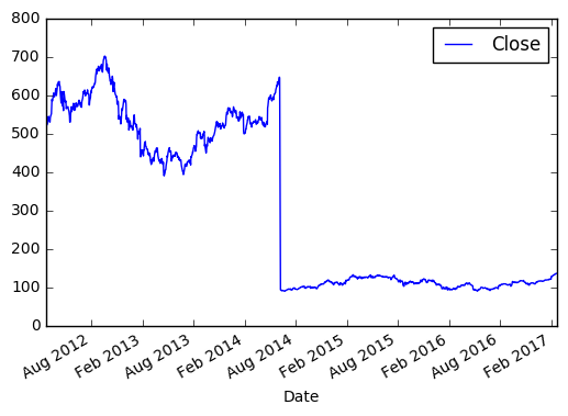
Values of X-axis are represented by index values of DataFrame (by default if you do not provide explicitly), Y-axis is a closing price. Take a look at 2014, there is a drop because of 7 to 1 split held by Apple.
That’s it for the introduction to pandas. Hope you like it, if so please leave a comment below.